Investigation of Clouds fromGround-based
and Airborne Radar and Lidar (CARL)
Contribution of the University of Athens (NKUA)
1. Introduction
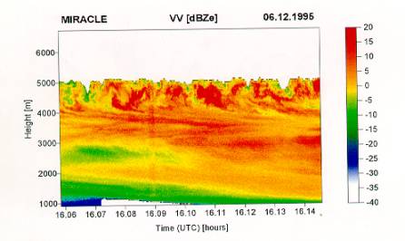
On 6 December 1995 the GKSS 95 GHz cloud radar located
at Geestacht, northern Germany (called the region of interest hereafter)
detected a cloud layer at the layer 4000-5000 m for the time interval 1606 UTC
to 1614 UTC (Fig. 1). Although the period of observations was very short (8
minutes), local observers reported that this cloud layer covered the area
during almost all the day. This case has been selected as a test case in order
to investigate the ability of the Regional Atmospheric Modelling System (RAMS)
to resolve this cloud layer.
2. Synoptic
Setup
On 6 December 1995 a high pressure system prevails over Eastern Europe, which at 1200 UTC exceeds 1040 hPa over western Russia (Fig. 2a). This synoptic setting creates a weak southeasterly flow over central Europe and over the region of interest. Surface temperature is very low during the whole day over a major part of Europe, as low as -7 to -10°C over the area of interest. Light snow was also observed in many synoptic stations. The infrared satellite imagery at 1600 UTC 6 December (Fig. 2b) reveals the presence of medium level clouds over the area of interest, in good agreement with the radar observations, while over the Baltic Sea and offshore Latvia and Estonia, higher clouds are evident.
Figure 2: (a) Mean sea level pressure (at 5 hPa intervals),
valid at 1200 UTC 6 December 1995,
(b) false-colour infrared imagery from METEOSAT,
valid at 1600 UTC 6 December 1995.
3. Model Setup
The analysis of the cloud layer is based on nested-grid simulations performed with the Regional Atmospheric Modelling System. RAMS has been developed at Colorado State University as a research model, but recently is starting also to be used as an operational model (e.g., Cotton et al., 1994; Tremback et al., 1994). A detailed description of the model physics and application fields is given in Pielke et al. (1992).
For the
present application, RAMS was initialised at 0000 UTC 06 December 1995 and the
duration of the simulation was 24 hours. The nonhydrostatic version of the
model is employed, while three nested grids have been defined. Indeed the
computational domain of the model consists of:
(a) the outer
grid, with a mesh of 76x62 points and 40 km horizontal grid interval centred at
53N latitude and 10E longitude
(b) the
second grid with 122x110 points and 10 km horizontal grid interval, centred at
53 41' N latitude and 10 42' E longitude.
(c) the inner grid with 82x82 points and 2,5 km horizontal grid interval, centred at 53 41' N latitude and 12 42' E longitude.
The inner
grid was introduced at 0900 UTC 06 December (after 9 hours of initialisation). The
horizontal extension of the grids is shown in Fig. 3. Twenty-eight levels
following the topography were used at the outer grid.
The vertical spacing varied from 120 m near the surface to 1000 m at the top of
the model domain. Vertical nesting was applied to the second and third grid,
permitting to resolve adequately the cloud layer. Indeed from 1750 to 9300 m,
18 extra vertical levels were used with approximately 250-300 m vertical
resolution. Along with these settings, other RAMS configuration options include:
The lateral boundary conditions on the outer grid were the relaxation scheme similar to Davies (1976).
A rigid lid has been set at the model top boundary
while top boundary nudging (which dumps gravity waves) has been activated.
A soil layer has been used to predict the sensible and latent heat fluxes at the soil-atmosphere interface (McCumber and Pielke, 1981; Avissar and Mahrer, 1988). Six soil levels have been used down to 50 cm below the surface.
The full microphysical package of RAMS has been activated (Walko et al, 1995). This package includes the condensation of water vapor to cloud water when supersaturation occurs as well as the prognosis of rain, graupel, pristine ice, aggregates, hail, and snow species.
A modified Kuo-type cumulus parametrization developed by Tremback (1990) is used because the model resolved convergence produced at the scales of the outer (40 km) grid is not enough to explicitly initiate convection.
A radiation scheme developed by Chen and Cotton (1983) which takes into account the influence of water vapor and condensate on shortwave nad longwave radiative transfer.
The ECMWF 0.5x0.5 gridded analysis
fields are objectively analysed by RAMS model on isentropic surfaces from which
they are interpolated to the RAMS grids, and they were used in order to
initialise the model. The 6-hourly ECMWF analyses were linearly interpolated in
time in order to nudge the lateral boundary region of the RAMS coarser grid at
a nudging time-scale of one hour. Moreover, the ECMWF analyses were blended
with all available surface and upper-air observations. Almost 80 upper-air
soundings and more than 1200 surface observations have been used at 6-hour
intervals. Observed sea-surface temperature data of 1x1 resolution provided by
ECMWF have been used. Moreover, topography derived from a 30"x30"
terrain data and gridded vegetation type data of 10'x10' resolution have been
used.
4. Model
results
This section
provides a short description of RAMS results during this event. Figure 4a
presents RAMS sea-level pressure and lowest model-level wind, valid at 1600 UTC
6 December. RAMS reproduces well the high pressure system over western Russia
(1045 hPa), as well as the weak easterly flow over Central Europe and
especially northern Germany where the radar was operating. The wind intensity
was about 8 ms-1 over the area of interest, while the flow is
accelerated over the North Sea, exceeding 16 ms-1.
Figure
4: (a) Mean sea-level pressure (at 5 hPa intervals) and wind field at the
lowest model level, on the outer grid of RAMS, valid at 1600 UTC 6 December
1995, (b) as in (a) except for temperature (at 2 °C intervals). Negative values are dashed.
RAMS
temperature field at the lowest model level (Fig. 4b) reproduces fairly well
the negative temperature values characterizing the major portion of the domain,
with values of about -6 °C in northern Germany and less than -8 °C in
central Germany. Indeed, temperature records at Hamburg (denoted by H in Fig.
4b) and at Erfurt (denoted by E at Fig. 4b) reported -5.8 °C and
-7 °C,
respectively, while the reported wind at Hamburg is from eastern direction,
with an intensity of 8 ms-1 at 1600 UTC, in very good agreement with
RAMS results (see Fig. 4a).
Figure
5: Vertical cross section inside the second grid of RAMS, following line AB in
Fig. 3, valid at 1600 UTC 6 December 1995 of (a) ice mixing ratio (g/kg), (b)
pristince ice mixing ratio (g/kg).
A series of vertical cross sections inside the second
grid of RAMS (following line AB in Fig. 3), permits to assess the vertical
structure of condensates over the area of interest. Figure 5a presents a
vertical cross section of ice mixing ratio at 1600 UTC, bounded vertically at 7
km. Over the western part of the domain, the whole atmospheric depth shown in
Fig. 5a is characterised by high concentrations of ice, while on the eastern
part of the domain a well defined layer of ice condensates is evident within
the layer 4 to 5 km, in good agreement with the radar observations (Fig. 1).
The cloud layer is also evident in the cross-section of the pristine ice mixing
ratio, where a well defined layer of high values of pristine ice covers
the eastern part of the domain shown (Fig. 5b).
In order to
compare model-generated clouds with the satellite imagery, ice water path (IWP
hereafter) can be used as a surrogate of upward longwave radiation (Heckman and
Cotton, 1993). Ice water path can be defined as:

where ri
is the ice mixing ratio and r is the air density. This quantity, integrated over a
certain layer of the atmosphere, is a
measure of optical thickness. In order to compare the vertical position of
clouds, the atmosphere was splited into two layers: 0-6 km and 6-16 km. This
splitting permits to identify lower/middle clouds and higher clouds. Figures 6a
and 6b present ice-water path within two layers over the second grid of RAMS,
valid at 1600 UTC 6 December 1995.
Within the 0-6 km layer, IWP shows clouds over the area of interest, while
the region over the North Sea and the Baltic Sea is free from lower clouds
(Fig. 6a). Within the 6-16 km layer, IWP shows the absence of higher clouds
over the area of interest and the presence of high clouds over the Baltic Sea
and the Netherlands, in good agreement with the satellite imagery shown in Fig.
2b.
Figure 6: (a) Ice
water path within the layer 0-6 km, valid at 1600 UTC 6 December,
(b) as in (a) except for the layer 6-16 km.
5. Concluding remarks
On 6 December
1995, the GKSS polarimetric radar observed a well defined cloud band within the
layer 4-5 km. RAMS simulations succeeded to reproduce the general synoptic
situation, with the presence of a high
pressure system, a moderate easterly flow and very low surface temperature. The
activation of the full microphysics package of RAMS resulted in an accurate
reproduction of the cloud band within the layer seen by the radar, while the
ice-water path calculated by RAMS output presented a very good agreement with
the infrared satellite imagery.
It should be
noted here that the radar provided data over a very short time period (8
minutes), a fact which makes the comparison with the model results difficult.
During July 1998 the TRAC campaign took place near Paris and provided surface
and airborne radar and lidar measurements over a longer time period. Thus, an
event observed during TRAC will be selected in order to perform additional RAMS
simulations, as the available observations would be more appropriate for
comparison.
6. References
Avissar, R., and Y. Mahrer, 1988: Mapping frost sensitive areas
with a three dimensional local scale numerical model. Part I: Physical and
numerical aspects. J. Appl. Meteor.,
27, 400-413.
Chen,
C., and Cotton W.R., 1987: The physics of the marine stratocumulus-capped mixed
layer. Bound. Lay. Meteor., 25,
289-321.
Cotton,
W. B., T.Thompson and P.W. Mielke, 1994: Real time mesoscale prediction on
workstations. Bulletin Americ. Meteor.
Soc., 75, 349-362.
Davies,
H.C., 1976: A lateral boundary formulation for multi-level prediction models. Q. J. R. Meteor. Soc., 102, 405-418.
Heckman,
S.T., and W.R. Cotton, 1993: Mesoscale numerical simulation of cirrus
clouds-FIRE case study and sensitivity analysis. Mon. Wea.Rev., 121, 2264-2284.
McCumber
M.C., and R.A. Pielke, 1981: Simulation of the effects of surface fluxes of
heat and moisture in a mesoscale numerical model. Part I: Soil layer. J. Geophys. Res., 86, 9929-9938.
Pielke,
R.A, W.R. Cotton, R.L Walko, C.J. Tremback, W.A Lyons, L.D. Grasso, M.E.
Nicholls, M.D. Moran, D.A. Wesley, T.J. Lee, and J.H. Copeland, 1992: A
comprehensive meteorological modelling system - RAMS. Meteorol. Atmos. Phys., 49, 69-91.
Tremback,
C. J., 1990: Numerical simulation of a mesoscale convective complex: Model
development and numerical results. Ph.D. dissertation, Atmos. Sci. Paper No.
465, Colorado State University, Dept. of Atmos. Science, Fort Collins, Co 8523.
Tremback,
C. J., W.A. Lyons, W.R. Cotton, R.L. Walko, and B. Beitler, 1994: Operational
weather forecasting applications using the Regional Atmospheric Modelling
System (RAMS). Preprints of the 10th Conference on Numerical Weather
Prediction, Portland, OR, 18-22 July 1994.
Walko, R.L., W.R.
Cotton, M.P. Meyers and J.Y. Harrington, 1995: New RAMS cloud microphysics
parameterization. Part I: the single moment scheme. Atmos. Res., 38, 29-62.