4.Model
results
This section provides a short description of RAMS results during the
period 3-4May, which we considered as the most interesting period. Figure 5a
presents temperature and wind fields at 850 hPa, valid at 12:00 UTC 3 May, while
Figure 5b presents these fields, valid at 500 hPa.
The model reproduced fairly well the synoptic state over the model
domains. The same is true for the easterly flow over the central and northern
France (at 850 hPa) and the southeasterly flow (at 500 hPa) over the same area
where the radar was operating. As an
indication, the modeled wind speed at 12:00 UTC, at 850 hPa was about 8 m/s
with direction from 84 o. Measurements from radiosondes showed 7.8
m/s for the wind speed and 87o for its direction at 850 hPa. At 500
hPa the modeled wind speed was around 8 m/s from 170 o , while the sounding gave a value of 9 m/s
for the wind speed and 154o for its direction. RAMS temperature
fields reproduced fairly well the temperature values reported from the measurements.
As an indication, the temperature at 12:00 UTC was 8o C at 850 hPa
and -18o C at 850 hPa, according to the sounding during this time.
The estimated temperatures over the area of interest were 8 o C at
850 hPa and about -19 o C at 500 hPa.
(a)
(b)
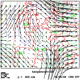

Figure 5: (a) temperature (at 1 C intervals and
wind field) at 500 hPa, on the outer grid of RAMS, valid at 12:00 UTC 3 May
1999, (b) as in (a) except at 850 hPa
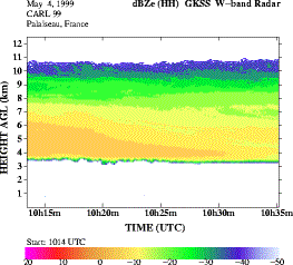
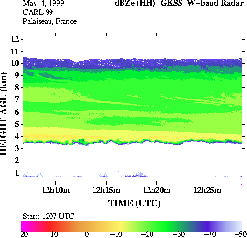
On 4 May the GKSS 95 GHz cloud radar
detected a cloud layer between 3.5 and 10 km (Fig.6a,6b). In figure 6c the
reflectivity measurements of the Lidar operations, at Palaiseau, is shown. As
we see a layer with water in liquid phase is evident at a layer near the ground
and between 4.5-5.5 km.
(a)
(b)
 ..
..
(c)
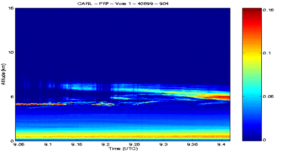
Figure 6: Reflectivity measurements (a),(b)
from the GKSS radar (c) from LIDAR
In order to compare the model
results with the observations a series of vertical cross-sections inside
the inner grid of RAMS (following line BA in Fig.4) were prepared. In these
cross-sections is defined the vertical structure of condensates over the area
of interest. Figures 7a, 7b and 8a present a vertical cross section of ice
mixing ratio at 07:00, 08:00 and 12:00 UTC respectively.
Palaiseau is located 40 km North
from the center of the outer domain and is indicated as '40' in the y axis of
the plots. Over the center of the domain a well defined layer of ice
condensates is evident. This is in good agreement with the radar observations.
The cloud layer is also evident in the cross-section of the pristine ice mixing ratio (fig. 8b and 9a), where a well defined layer of pristine ice covers all the domain, within the layer 7 to 11 Km at 09:00 UTC and 3 to 5 Km at 12:00 UTC.
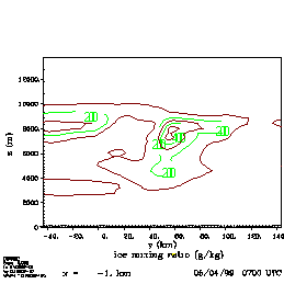
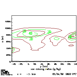
Figure 7: Vertical cross section inside the third grid of RAMS, following line AB in Figure 4, valid at 4 May 1999 of ice mixing ratio (g/kg) (a) at 07:00 UTC, (b) at 08:00 UTC. The labels in contours are multiplied by 10**5.
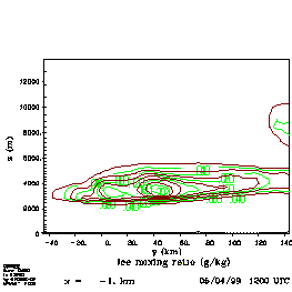
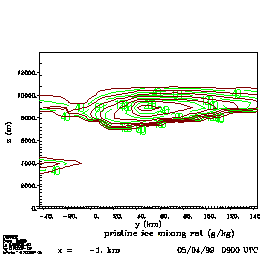
Figure 8: As in figure 7, but (a) mixing ratio (g/kg) at 12:00 UTC (b) pristine ice mixing ratio(g/kg) at 09:00 UTC. The labels in contours in (a) are multiplied by 1 while in (b) by 10**5.
Figures 9b and 10a present a
vertical cross-section of liquid mixing ratio at 09:00 UTC and 10:00 UTC
respectively, for the lower levels of the atmosphere, while figure 10a presents
liquid mixing ratio at 10:00 UTC for the middle levels. As shown in Figures 9b
and 10a the layer 0 to 500 m is characterized by high concentrations of water
in liquid phase for all the third grid of RAMS, while a smaller concentration
of liquid appears (Figure 10b), at the base of cloud, over the region of
interest, in good agreement with the lidar observations (Figure 6c)
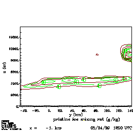
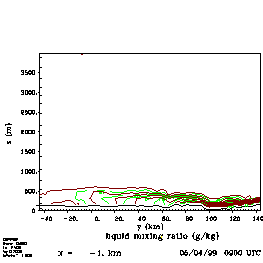
Figure 9: As in fig. 7 but (a)pristine ice mixing ratio at 12:00 UTC and (b) liquid mixing ratio (g/kg) at 09:00 UTC at the lower levels of the atmosphere. The contour labels in (a) are multiplied by 10**4 while in (b) are multiplied by 1.
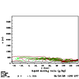
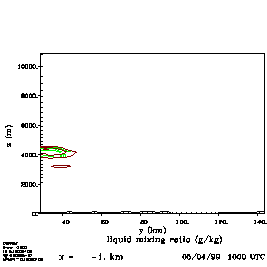
Figure 10: As in fig. 9 but (a)liquid mixing
ratio at 10:00 UTC at the lower levels and (b) liquid mixing ratio (g/kg) at
10:00 UTC at the upper levels of the atmosphere. The contour labels in (a) are
multiplied by 10**4 while in (b) are multiplied by 1.
In order to
compare model-generated clouds with the satellite imagery, ice water path (IWP
hereafter) can be used as a surrogate of upward longwave radiation (Heckman and
Cotton, 1993). Ice water path can be defined as:

ri is the ice mixing ratio and r is
the air density. This quantity, integrated over a certain layer of the
atmosphere, is a measure of optical thickness. In order to compare the vertical
position of clouds, the atmosphere was spited into two layers: 0-3 km and 3-12 km.
This splitting permits to identify lower clouds and higher clouds. Figures 11a
and b present the ice-water path within the layer 3-12 km for the second
and third grid of RAMS, for 12:00 UTC 5 May 1999. Within this layer, IWP shows
clouds over the area of interest, which is in good agreement with the
observations.
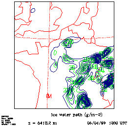

Figure
11: (a) Ice water path for the second grid within the layer 3-12 km, valid at
1200 UTC 4 May, (b) as in (a) except for the third grid.
The previously discussed results are with no nudging inside the grid domains. Several other sensitivity tests were performed with different nudging periods. In the sensitivity tests performed with nudging period of 3 hours, the cloud microphysical structure, which described previously are slightly modified. More specifically, the water in liquid phase was not evident in the cloud deck. This should lead us in the conclusion that some mesoscale structures are important in the cloud structures observed. The use of nudging option, in general, enhances the role of synoptic scale features and wipes out local structures.
5. Concluding remarks
Based on
the above, RAMS was able to reproduce satisfactorily the weather conditions
during the experimental period. The microphysical structure was simulated with
a satisfactory accuracy in general. The activation of the full microphysics
package of RAMS resulted in an accurate reproduction of the cloud band within
the layer, which has been also detected by the radar. This something which was
expected because microstructures are important in such large broad cloud
formation.
During
the next (third period) we will continue the analysis and the sensitivity tests
in order to explore possible model improvements and other sensitivities. Then,
simulations for the remaining days (5-7 May) will be performed. The simulations
will be repeated with a new version of RAMS (version 4.2) where an improved
cloud microphysical scheme is implemented.
6. References
Avissar, R., and
Y. Mahrer, 1988: Mapping frost sensitive areas with a three dimensional local
scale numerical model. Part I: Physical and numerical aspects. J. Appl. Meteor., 27, 400-413.
Chen, C., and Cotton W.R.,
1987: The physics of the marine stratocumulus-capped mixed layer. Bound. Lay. Meteor., 25, 289-321.
Cotton, W. B., T.Thompson
and P.W. Mielke, 1994: Real time mesoscale prediction on workstations. Bulletin Americ. Meteor. Soc., 75,
349-362.
Davies, H.C., 1976: A
lateral boundary formulation for multi-level prediction models. Q. J. R. Meteor. Soc., 102, 405-418.
Heckman, S.T., and W.R. Cotton, 1993: Mesoscale numerical simulation
of cirrus clouds-FIRE case study and sensitivity analysis. Mon. Wea.Rev., 121, 2264-2284.
McCumber M.C., and R.A.
Pielke, 1981: Simulation of the effects of surface fluxes of heat and moisture
in a mesoscale numerical model. Part I: Soil layer. J. Geophys. Res., 86, 9929-9938.
Pielke, R.A, W.R. Cotton,
R.L Walko, C.J. Tremback, W.A Lyons, L.D. Grasso, M.E. Nicholls, M.D. Moran,
D.A. Wesley, T.J. Lee, and J.H. Copeland, 1992: A comprehensive meteorological
modelling system - RAMS. Meteorol. Atmos.
Phys., 49, 69-91.
Tremback, C. J., 1990:
Numerical simulation of a mesoscale convective complex: Model development and
numerical results. Ph.D. dissertation, Atmos. Sci. Paper No. 465, Colorado
State University, Dept. of Atmos. Science, Fort Collins, Co 8523.
Tremback, C. J., W.A. Lyons,
W.R. Cotton, R.L. Walko, and B. Beitler, 1994: Operational weather forecasting
applications using the Regional Atmospheric Modelling System (RAMS). Preprints
of the 10th Conference on Numerical Weather Prediction, Portland, OR, 18-22
July 1994.
Walko, R.L., W.R. Cotton, M.P. Meyers and
J.Y. Harrington, 1995: New RAMS cloud microphysics parameterization. Part I:
the single moment scheme. Atmos. Res.,
38, 29-62.