Investigation of cloud by ground-based and airborne Radar and Lidar (CARL)
The
first European CARL intensive experiment was held in France during the spring
(April-May) of 1999 on the experimental site of IPSL at Palaiseau (near Paris).
It was devoted to measurements in ice clouds and involved ground-based lidar,
radar and radiometry measurements as well as in situ validation measurements
from aircraft. Preparation of the campaign was done by IPSL/LMD. In situ
measurements were obtained using the
GKSS sondes installed on one of the aircraft of Meteo-France. Ground-based
lidar and radar measurement were taken by IPSL and GKSS. Airborne measurements
were taken during AVHRR overpasses to allow complementary analysis using
space-borne radiometry. Additional ground-based radiometry measurements were
made by KNMI. Mesoscale modeling has
also been started by NKUA / AM&WFG on the priority case of 4 May.
Modeling Analysis
Model setup
For the present application,
RAMS ( the new version 4.2.9) was initialized at 0000 UTC 03 May 1999. The
duration of the simulation was 48 hours. The non-hydrostatic version of the
model was employed, with three nested grids. The computational domain of the
model consists of:
a) the outer grid, with a mesh
of 110x94 points and 45 km horizontal
grid interval centered at 48o N latitude and 17 o E
longitude
b) the second grid with 83x74
points and 15 km horizontal grid interval centered at 48 o 44 N
latitude and 2 o 15 E longitude
c) the inner grid with 86x86 points
and 2.5 km horizontal grid interval centered at the same point with the second
grid (over Palaiseau)
The horizontal extension
of the grids is shown in figure 1. For the outer grid 31 vertical levels
following the topography were used. The vertical spacing varied from 110m near
the surface to 1000 m at the top of the model domain.
Vertical nesting was
applied to the second and third grid, permitting adequate resolution the cloud
layer. For these grids were used 36 vertical levels. Along with these settings,
other RAMS configuration options include:
a) The lateral boundary
conditions to the outer grid where the scheme similar to Klemp/Wilhelmson.
b) A rigid lid was set at
the model top boundary while top boundary nudging (which dumps gravity waves)
was activated.
c) A soil layer was used to
predict the sensible and latent heat fluxes at the soil-atmosphere interface.
Eight soil levels were used down to 1.2 m below the surface.
d) The full microphysical package of RAMS was
activated. This package includes the condensation of water vapor when
supersaturation occurs as well as the prognosis of rain, graupel, pristine ice,
aggregates, hail and snow species.
e) A modified Kuo-type
cumulus parametarization developed by
Tremback( 1990) was used because the model resolved convergance produced at the
scales of the outer (45 Km) grid, is not enough to explicitly initiate
convection.
f) A radiation scheme
developed by Chen and Cotton (1983) which takes into account the influence of
water vapor and condensate on shortwave and longwave radiative transfer was
used.
The ECMWF 0.5ox0.5o gridded analysis fields was objectively
analysed by RAMS model on isentropic surfaces from which they are interpolated
to the RAMS grids . These data were used in order to initialize the model.
(a) (b) (b) Figure 1: The three nested grid of RAMS. a)
the first grid b) the second and the third grid ( green color ) The RAMS model
was run by NKUA for the 3 and 4 May to reproduce the synoptic state over the
model domains. Figures 1 and 2 present temperature and wind fields obtained at 850hPa and 500 hPa
respectively, valid at 12:00 UTC 3 May. These figures exhibit southeasterly
flow over France at the lower tropospheric layers and southerly flow at the
middle tropospheric layers. Figures 3 and 4 present the same fields at the same
pressure levels, valid at 12:00 UTC, 4 May. RAMS reproduced fairly well the
observed temperature and wind fields. Figure 2: Wind field and temperature (at 2oC
intervals) at 850 hPa, valid at 12:00 UTC 3 May 1999. Figure 3: As in figure 1 but at 500 hPa Figure 4: Wind field and temperature (at 2oC
intervals) at 850 hPa, valid at 12:00 UTC 4 May 1999. Figure 5: As in figure 1, but at 500 hPa In order to compare the model
results with the observations a series of time-height plots, horizontal plots
and latitudinal cross-sections, inside the inner grid of RAMS, over Palaiseau ( latitude:48o 43 ,
longitude:2o 15 ), have been prepared. Time-height plots of: U-component
of wind, V-component of wind, W-component of wind, turbulent kinetic energy,
equivalent potential temperature, pressure, vapor mixing ratio, and
temperature. All the heights are above ground level (AGL). Figure 6: U-wind (m/s) Figure 7: V-wind (m/s) Figure 8: W-wind (m/s) Figure 9: Turbulent kinetic energy (m2/s2) Figure 10: Equivalent potential temperature
(o Kelvin) Figure 11: Wind speed (m/s) Figure 12: vapor mixing ratio (g/kg) Figure 13: Temperature (o
C) Time-height
plots of microphysical parameters. All heights are above ground level ( AGL ) Figure 14: Pristine ice concentration
per volume (#/l) Figure 15: Pristine ice diameter
(microns) Figure 16: Pristine ice mass per
volume (mg/l) Figure 17: Snow concentration per
volume (#/l) Figure 18: Snow diameter (mm) Figure 19: Snow mass per volume
(mg/l) Figure 20: Aggregates concentration
per volume (#/l) Figure 21: Aggregates diameter (mm) Figure 22: Aggregates mass per volume
(mg/l) Figure 23: Graupel concentration per volume (#/m3) Figure 24: Graupel diameter (mm) Figure 25: Graupel mass per volume (micrograms/l) Figure 26: Hail concentration per
volume (#/m3) Figure 26: Hail diameter (mm) Figure 27: Hail mass per volume
(micrograms/l) Figure 28: Rain droplets
concentration per volume (#/l) Figure 29: Rain diameter (mm) Figure 30: Rain mass per volume
(mg/l) Figure 31: Cloud droplets mass per
volume (mg/l) Figure 32: Total ice mass per volume
(mg/l) Figure 33: Total liquid mass per
volume (mg/l) Plots from the GKSS W-band Radar Figure 34: Reflectivity
measurements from the GKSS radar Latitudinal cross-sections of microphysical parameters In addition a series of latitudinal
cross-sections inside the inner grid of
RAMS, following the line AB in figure 1, has been prepablack. In these
cross-sections the vertical structure of condensates has been defined over the
area of interest. While the plots has been made parallel to 2o 15
longitude, Palaiseau is located 630 km North from the center of the outer
domain and is indicated as ‘630’ in the y axis of the plots. Some of these
plots are shown below. A number of these cross-sections valid at 4 May 1999(13:00 UTC), are defined below. (a) (b) (c) Figure 35: (a) aggregates concentration per
volume (#/L), (b) aggregates diameter (mm) and (c) aggregates mass per volume
(mg/L) (a) (b) (c ) Figure 36: (a) graupel concentratrion per volume (#/m3) , (b) graupel
diameter (mm) and (c ) graupel mass per volume (micrograms/L) (a) (b) (c) Figure 37: (a) hail concentration per volume (#/m3), (b) hail diameter (mm) and
(c) hail mass per volume (micrograms/L) (a) (b) (c) Figure 38: (a) pristine ice concentration per volume (#/L), (b) pristine ice
diameter (microns) and (c) pristine mass per volume (mg/L) (a) (b) (c) Figure 39: (a) rain concentration per volume (#/L), (b) rain diameter (mm)
and (c) rain mass per volume (mg/L) (a) (b) (c) Figure 40: (a) snow concentration per volume (#/L), (b) snow diameter (mm) and
(c) snow mass per volume (mg/L) (a) (b) (c) Figure 41: (a) total ice mass per volume
(mg/L), (b) total liquid mass per volume (mg/L) and (c) cloud droplets mass per
volume (mg/L) Also horizontal plots has been made
for surface heat and Radiative fluxes. Palaiseau is located 630 km North and
1080 km West from the center of the outer domain and is indicated as "630" in
the Y-axis and "-1080" in the X-axis of the plots. (a) (b) (c) (d) Figure 42: Latent heat flux (w/m2) valid at 4
May (a) at 9:00 UTC, (b) at 11:00 UTC, (c) at 13:00 UTC and (d) at 15:00 UTC (a) (b) (c) (d) Figure 43: Sensible heat flux (w/m2) valid at
4 May (a) at 9:00 UTC, (b) at 11:00 UTC, (c) at 13:00 UTC and (d) at 15:00 UTC (a) (b) (c) (d) Figure 44: Shortwave radiative fluxes valid at 4 May (a) at 9:00
UTC, (b) at 11:00 UTC, (c) at 13:00 UTC and (d) at 15:00 UTC (a) (b) (c) (d) Figure 45: Downwards longwave radiative fluxes valid at 4 May (a) at 9:00
UTC, (b) at 11:00 UTC, (c) at 13:00 UTC and (d) at 15:00 UTC (a) (b) (c) (d) Figure 46: Upwards longwave radiative fluxes valid
at 4 May (a) at 9:00 UTC, (b) at 11:00 UTC, (c) at 13:00 UTC and (d) at 15:00
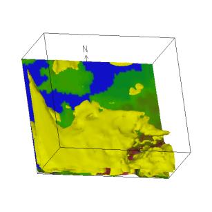
UTC Figure 47: A three-dimensional
illustration of the 90 percent iso-surface of relative humidity at the first domain,
seen from the top, valid at 8:00 UTC 4 May 1999. Figure
48:
a) A three-dimensional illustration of the 90 percent iso-surface of relative
humidity at the second domain, valid at 8:00 UTC, 4 May 1999 and b) the same as
(a) but seen from the west. More graphics for model output are currently been
under construction!!! 
Synoptic setup
Model results


Horizontal
plots

Three dimensional plots