Investigation of Clouds from Ground-based
and Airborne Radar and Lidar (CARL)

Contribution of the University of Athens (NKUA)

1. Introduction

After an agreement among the partners (May 4 1999 at Palaiseau), the new RAMS simulations for the reporting period will be during the experimental campaign at Palaiseau (called the region of interest hereafter). This experimental campaign was performed during 3-7 May 1999. Several tests were performed with a number of various model configurations. We briefly present the results of the last simulation as well as some sensitivity tests.

2. Synoptic Setup

The synoptic conditions occurring during the experimental period 3-7 May are summarized as follows:

On May 3, a South-southeasterly flow was evident over the gulf of Genoa (Fig. 1a). An easterly flow was observed over central and northern France at the lower tropospheric layers 850 hPa and 700 hPa(not shown here). During this day, southeasterly flow dominated the middle tropospheric layers (500 hPa) over Central France (Fig. 1b). During the next day, the winds over the gulf of Genoa were backing to the east (Fig. 2a), while the flow over Central and South France was northerly(1000 hPa). Over the region of interest the synoptic situation created a southeasterly flow at 500 hPa. (Fig. 2b). Thus there was cooling near surface and warming aloft. This warming caused a partial melting near the bottom cloud layers. Fig. 3 shows the water content in the mid-tropospheric layer of 500 hPa. As it is seen, the water content was increased on May 4.

(a)

Figure 1a: Wind field and temperature (at 2 ^oC intervals) at 1000 hPa, valid at 12:00 UTC 3 May 1999.

(b)

Figure 1b : As in fig. 1a except for 500 hPa

(a)

(b)

Figure 2: As in fig. 1 except for 4 May 1999

(a) (b)

Figure 3: Vapor mixing ratio (g/kg) at 500 hPa (a) valid at 3 May 1999 (b) valid at 4 May

3. Model Setup

For the present application, RAMS was initialised at 0000 UTC 03 May 1999 The duration of the simulation was 48 hours. The non-hydrostatic version of the model was employed, with three nested grids. The computational domain of the model consists of:

(a) the outer grid, with a mesh of 76x62 points and 40 km horizontal grid interval centred at 48°N latitude and 2° 15 ' E longitude

(b) the second grid with 122x110 points and 10 km horizontal grid interval, centred at 48° 44 ' N latitude and 2° 15 ' E longitude (over Palaiseau).

(c) the inner grid with 82x82 points and 2,5 km horizontal grid interval, centred at 48° 44 ' N latitude and 2° 15' E longitude (over Palaiseau).

The horizontal extension of the grids is shown in Fig. 4. Twenty-five vertical levels following the topography were used for the outer grid. The vertical spacing varied from 120 m near the surface to 1000 m at the top of the model domain. Vertical nesting was applied to the second and third grid, permitting adequate resolution the cloud layer. From 1300 to 10800 m, 18 extra vertical levels were used with approximately 200-350 m vertical spacing. Along with these settings, other RAMS configuration options include:

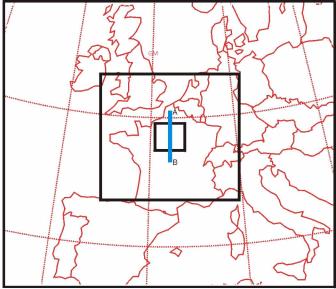
Figure 4: Extension of the three nested grid of RAMS

· The lateral boundary conditions on the outer grid were the relaxation scheme similar to Davies (1976).

· A rigid lid was set at the model top boundary while top boundary nudging (which dumps gravity waves) was activated.

· A soil layer was used to predict the sensible and latent heat fluxes at the soil-atmosphere interface (McCumber and Pielke, 1981; Avissar and Mahrer, 1988). Six soil levels were used down to 50 cm below the surface.

· The full microphysical package of RAMS (Walko et al, 1995) was activated. This package includes the condensation of water vapor to cloud water when supersaturation occurs as well as the prognosis of rain, graupel, pristine ice, aggregates, hail, and snow species.

· A modified Kuo-type cumulus parametrization developed by Tremback (1990) was used because the model resolved convergence produced at the scales of the outer (40 km) grid is not enough to explicitly initiate convection.

· A radiation scheme developed by Chen and Cotton (1983) which takes into account the influence of water vapor and condensate on shortwave and longwave radiative transfer was used.

The ECMWF 0.5°x0.5° gridded analysis fields are objectively analysed by RAMS model on isentropic surfaces from which they are interpolated to the RAMS grids, This data was used in order to initialise the model. The 6-hourly ECMWF analyses were linearly interpolated in time in order to nudge the lateral boundary region of the RAMS coarser grid at a nudging time-scale of one hour. Moreover, the ECMWF analyses were blended with all available surface and upper-air observations. Almost 60 upper-air soundings and more than 900 surface observations was used (at 6- hour intervals). Climatological sea-surface temperature data of 1°x1° resolution was used. In addition, topography was derived from a 30"x30" terrain data and gridded vegetation type data of 30"x30" resolution.

The atmospheric model solution is relaxed toward the analyzed data during time integration. The strength of the nudging is given by ( I -M) /T. I is an initialization file data value at a particular location, M is the corresponding model value, and T is a user-specified relaxation time scale.

Several sensitivity tests were performed, for domain selection, grid resolution, size vertical layering etc. As we found the most crucial parameter is the nudging time period. Some of these results are discussed below.

For more (click here)